2. Backtracking 1-step diagram - manual
The LaTeX in this section is for a 1-step backtracking diagram.
The values in the diagram can be entered manually into the LaTeX code.
The snippet below from the LaTeX file shows a block in the preamble of the .tex file where the values for the backtacking diagram can be manually edited.
The values,
x, 2x, 6, 3 in the braces {} can be altered.The processes,
\times2 and \div2 can be replaced with + and -.% modify values for backtracking
\def\stepAB{\times2}
\def\stepABrev{\div2}
\def\boxA{x}
\def\boxB{2x}
\def\boxBrev{6}
\def\boxArev{3}
% end modify values for backtracking
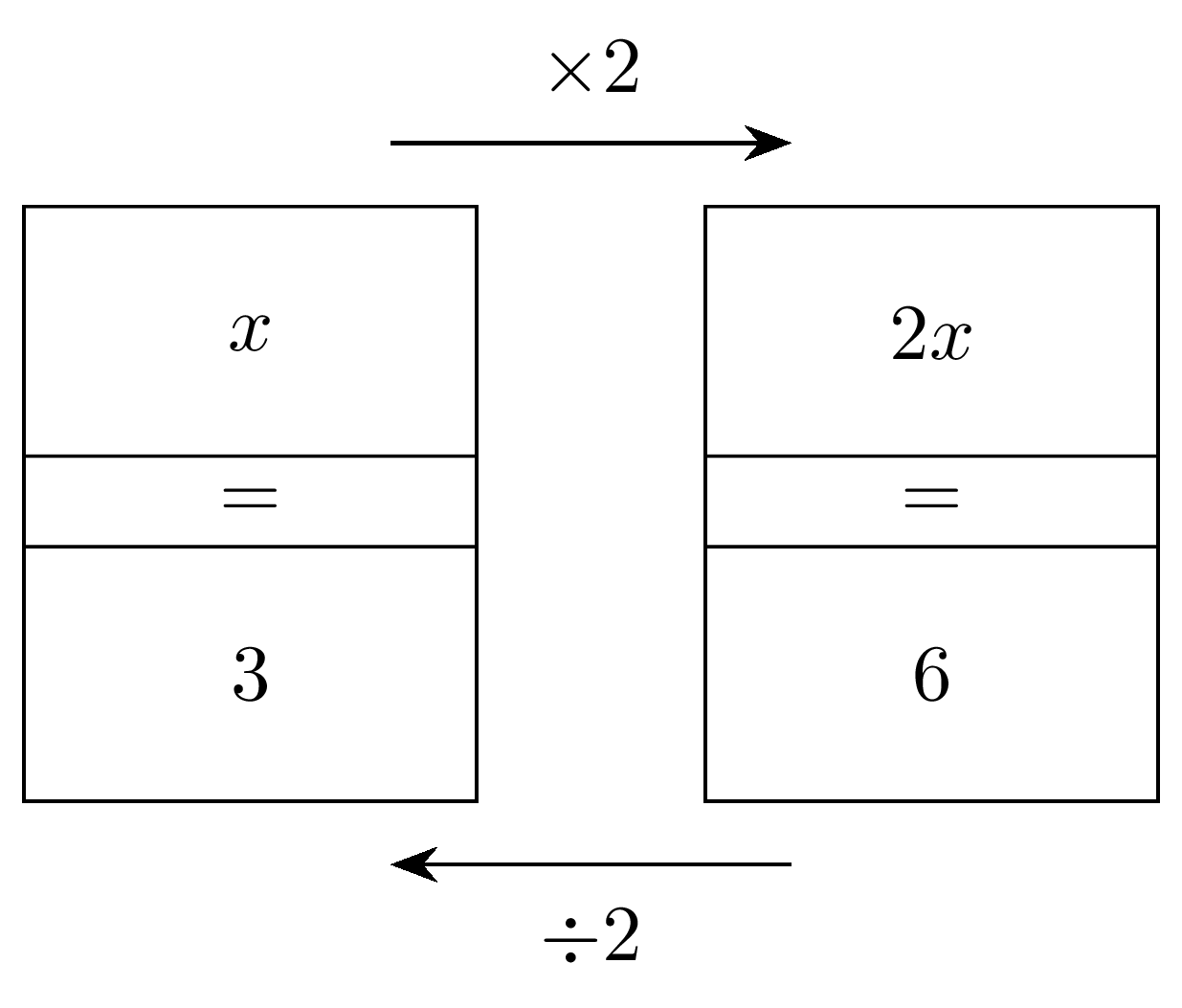
2.1. A 1-step backtracking diagram with answers


2.2. 1-step backtracking LaTeX
A LaTeX .tex file consists of two parts, the preamble and the main document.
2.3. LaTeX preamble
In the preamble, set the document class, and import required packages and set their options.
Macro definitions, such as those for the variables to hold the diagram values, are also in the preamble.
\documentclass[border = 1mm]{standalone}
\usepackage{tikz}
\usetikzlibrary{positioning}
\usetikzlibrary {arrows.meta}
\tikzset{backtrack/.style={rectangle,draw=black,fill=white,
inner sep=2pt,minimum height=32pt, minimum width=20mm}}
\tikzset{backtrackeq/.style={rectangle,draw=black,fill=white,
inner sep=2pt,minimum height=12pt, minimum width=20mm}}
\tikzset{backtrackstep/.style={rectangle,draw=none,fill=white,
inner sep=2pt,minimum height=12pt, minimum width=20mm}}
% modify values for backtracking
\def\stepAB{\times2}
\def\stepABrev{\div2}

\def\boxA{x}
\def\boxB{2x}
\def\boxBrev{6}
\def\boxArev{3}
% end modify values for backtracking
2.3.1. Document class
The code
\documentclass[border = 1mm]{standalone} is used to define a document that can be used to create graphics that are self-contained and can be easily included in other documents.The argument [border = 1mm] specifies the size of the border around the content of the document.
2.3.2. tikz package
The code
\usepackage{tikz} imports the TikZ package which allows you to create diagrams and graphics programmatically, such as points, lines and paths, circles, ellipses and rectangles.The code
\usetikzlibrary{positioning} is used to import the positioning library which provides advanced positioning options for nodes (points in a diagram that can be referenced and used to draw lines or shapes).For docs on the tikz package see: https://tikz.dev/
2.3.3. tikzset for styles
Styles are set so that applying the same style to multiple parts of the diagram is more efficient.
This line
\tikzset{backtrack...}} defines a new style called backtrack for rectangles in TikZ.The style is defined with the following properties:
rectangle: The shape of the node is a rectangle.
draw=black: The border color of the rectangle is black.
fill=white: The fill color of the rectangle is white.
inner sep=2pt: The distance between the border and the content of the node is 2pt.
minimum height=32pt: The minimum height of the rectangle is 32pt.
minimum width=20mm: The minimum width of the rectangle is 20mm.
\tikzset{backtrack...} defines the top and bottom rectangle features.\tikzset{backtrackeq...} defines the middle rectangle features.\tikzset{backtrackstep...} defines the step features of the text on an arrow.2.3.4. Macro definitions
The variables to be used are shown below in the Macro definitions.
These will be used in creating the backtracking diagram.
This allows a user to replace the values that show on the backtracking diagram, here, in one place, instead of in the LaTeX code for the diagram itself.
% modify values for backtracking
\def\stepAB{\times2}
\def\stepABrev{\div2}

\def\boxA{x}
\def\boxB{2x}
\def\boxBrev{6}
\def\boxArev{3}
% end modify values for backtracking
2.3.5. Macro definitions and Variables
The command
\def is used to define new commands in LaTeX.The syntax for defining a new command is
\def\commandname{replacement text}.When the command is used in the document, LaTeX replaces it with the replacement text.
The command
\def\stepAB{\times2} defines a new command named, \stepAB, that takes no arguments and expands to the text \times2. i.e. sets the value of the variable, stepAB, to {\times2}.Later in the code,
{$\stepAB$} allows the variable value, \times2 to be placed in the diagram. It appears as “x2”.The 1-step backtracking diagram shows the names of the variables used for each part of the diagram.

2.3.5.1. The document environment
The tikzpicture part of the document environment is below.
It contains nodes with names to identify each position used to draw lines and rectangles.
\begin{document}

\begin{tikzpicture}
    \node[backtrack] (boxA) at (0, 0) {$\boxA$};
    \node[backtrack] (boxB) [right=1cm of boxA] {$\boxB$};

    \node[backtrackeq] (boxAeq) [below=-1pt of boxA] {$=$};
    \node[backtrackeq] (boxBeq) [below=-1pt of boxB] {$=$};

    \node[backtrack] (boxArev) [below=-1pt of boxAeq] {$\boxArev$};
    \node[backtrack] (boxBrev) [below=-1pt of boxBeq] {$\boxBrev$};

    \node (boxAr) at ([yshift=24pt,xshift=5mm]boxA) { };
    \node (boxBl) at ([yshift=24pt,xshift=-5mm]boxB) { };
    \draw [line width=0.4pt,-{Stealth[length=2mm]}] (boxAr)  --node[backtrackstep,above=2pt] {$\stepAB$} (boxBl);

    \node (boxBrevl) at ([yshift=-24pt,xshift=-5mm]boxBrev) { };
    \node (boxArevr) at ([yshift=-24pt,xshift=5mm]boxArev) { };
    \draw [line width=0.4pt,-{Stealth[length=2mm]}] (boxBrevl)  --node[backtrackstep,below=2pt] {$\stepABrev$} (boxArevr);

\end{tikzpicture}

\end{document}
2.3.6. Document
The command
\begin{document} starts the body of the document. It is used to indicate the beginning of the text that will be typeset to appear in the output pdf.The
\end{document} command marks the end of the document2.3.7. tikzpicture
\begin{tikzpicture} is a command in LaTeX that creates a new picture environment.2.3.8. Nodes
A node is a point in a diagram that can be referenced and used to draw lines or shapes.
Nodes are created using the syntax ``node[<options>] (<name>) at (<coordinate>) {<text>}``.
The
<options> are optional and can be used to customize the node’s appearance.The
<name> is also optional and can be used to reference the node later.The
<coordinate> specifies the position of the node in the diagram.The
<text> is the text that appears inside the node.See syntax for nodes at: https://tikz.dev/tikz-shapes
The command
\node[backtrack] (boxA) at (0, 0) {$\boxA$} creates a node, named boxA, with the style backtrack at position (0, 0) and with the content given by the variable \boxA.The command
\node[backtrack] (boxB) [right=1cm of boxA] {$\boxB$} creates a node with the style backtrack, positioned 1cm to the right of another node 1cm to the right of node named boxA and with text inside the node given by the variable \boxB.The command
\node[backtrackeq] (boxAeq) [below=-1pt of boxA] {$=$} creates a node with the style backtrackeq, placed 1pt below the node boxA with the text “=” inside the node .The command
\node (boxAr) at ([yshift=24pt,xshift=5mm]boxA) { } creates a node named boxAr at a position that is 24pt above and 5mm to the right of the node named boxA. The node is empty, so it doesn’t contain any text.The command
\draw [line width=0.4pt,-{Stealth[length=2mm]}]] (boxAr) --node[backtrackstep,above=1pt] {$\stepAB$} (boxBl) is used to draw an arrow from the node boxAr to the node boxBl.The draw option
[line width=0.4pt,-{Stealth[length=2mm]}]] draws a stealth arrow using the “Stealth” arrowhead. The arrow has a width of 0.4 point (which is very narrow) and a length of 2 mm. The arrowhead is a stealth shape, which has a pointed tip with a long shaft and a small head. It’s commonly used in technical drawings.For more on arrows see: https://tikz.dev/tikz-arrows.
The text value of the variable
\stepAB is placed above the arrow.2.3.9. Font size
The default font size for most of the standard document classes in LaTeX is 10pt.
The font size options for most document classes are 10pt, 11pt, and 12pt.
This size becomes the setting for
\normalsize option, and all the other size commands are adjusted accordingly.If you want to change the font size locally, you can use predefined commands such as
\Large, \Large, \LARGE, \Large, \large, \normalsize, \small, \footnotesize, \scriptsize, and \tiny.2.4. 1-step backtracking LaTeX
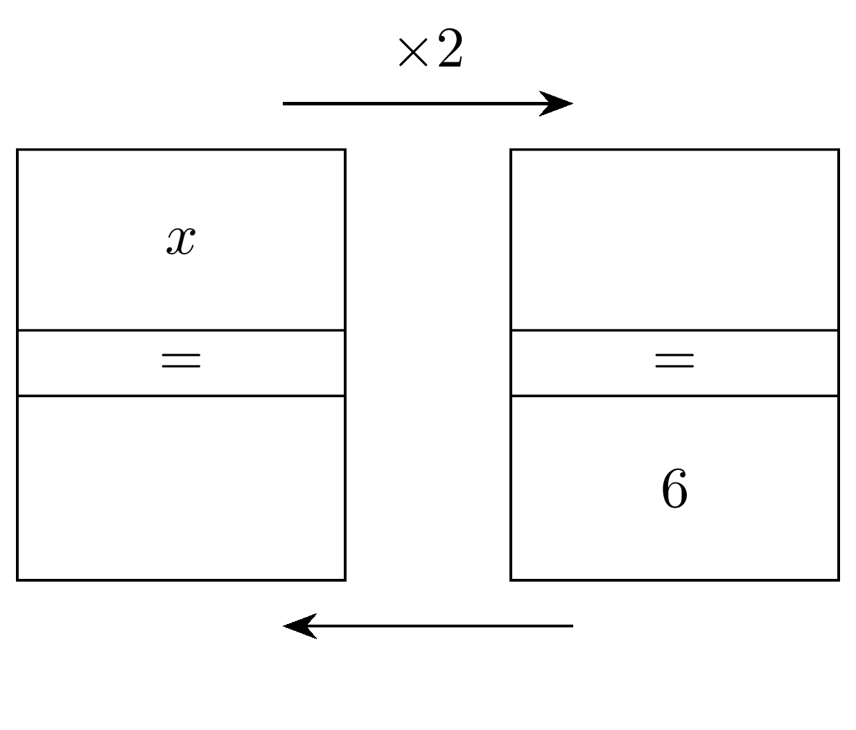
The 1-step backtracking LaTeX for the question (incomplete) diagram is below.
Some variable values have been commented out and replaced with empty values.
 1% backtracking diagrams
 2\documentclass[border = 1mm]{standalone}
 3\usepackage{tikz}
 4\usetikzlibrary{positioning}
 5\usetikzlibrary {arrows.meta}
 6
 7\tikzset{backtrack/.style={rectangle,draw=black,fill=white,
 8inner sep=2pt,minimum height=32pt, minimum width=20mm}}
 9\tikzset{backtrackeq/.style={rectangle,draw=black,fill=white,
10inner sep=2pt,minimum height=12pt, minimum width=20mm}}
11\tikzset{backtrackstep/.style={rectangle,draw=none,fill=white,
12inner sep=2pt,minimum height=12pt, minimum width=20mm}}
13
14
15% modify values for backtracking
16% comment out values for question diagram
17\def\stepAB{\times2}
18\def\stepABrev{} % {\div2}
19
20\def\boxA{x}
21\def\boxB{} %2x}
22\def\boxBrev{6}
23\def\boxArev{} % {3}
24% end modify values for backtracking
25
26
27
28\begin{document}
29
30\begin{tikzpicture}
31    \node[backtrack] (boxA) at (0, 0) {$\boxA$};
32    \node[backtrack] (boxB) [right=1cm of boxA] {$\boxB$};
33
34    \node[backtrackeq] (boxAeq) [below=-1pt of boxA] {$=$};
35    \node[backtrackeq] (boxBeq) [below=-1pt of boxB] {$=$};
36
37    \node[backtrack] (boxArev) [below=-1pt of boxAeq] {$\boxArev$};
38    \node[backtrack] (boxBrev) [below=-1pt of boxBeq] {$\boxBrev$};
39
40    \node (boxAr) at ([yshift=24pt,xshift=5mm]boxA) { };
41    \node (boxBl) at ([yshift=24pt,xshift=-5mm]boxB) { };
42    \draw [line width=0.4pt,-{Stealth[length=2mm]}] (boxAr)  --node[backtrackstep,above=3.0pt] {$\stepAB$} (boxBl);
43
44    \node (boxBrevl) at ([yshift=-24pt,xshift=-5mm]boxBrev) { };
45    \node (boxArevr) at ([yshift=-24pt,xshift=5mm]boxArev) { };
46    \draw [line width=0.4pt,-{Stealth[length=2mm]}] (boxBrevl)  --node[backtrackstep,below=3.0pt] {$\stepABrev$} (boxArevr);
47
48\end{tikzpicture}
49
50\end{document}
The 1-step backtracking LaTeX for the answer (complete) diagram is below.
 1% backtracking diagrams
 2\documentclass[border = 1mm]{standalone}
 3\usepackage{tikz}
 4\usetikzlibrary{positioning}
 5\usetikzlibrary {arrows.meta}
 6
 7\tikzset{backtrack/.style={rectangle,draw=black,fill=white,
 8inner sep=2pt,minimum height=32pt, minimum width=20mm}}
 9\tikzset{backtrackeq/.style={rectangle,draw=black,fill=white,
10inner sep=2pt,minimum height=12pt, minimum width=20mm}}
11\tikzset{backtrackstep/.style={rectangle,draw=none,fill=white,
12inner sep=2pt,minimum height=12pt, minimum width=20mm}}
13
14
15% modify values for backtracking
16\def\stepAB{\times2}
17\def\stepABrev{\div2}
18
19\def\boxA{x}
20\def\boxB{2x}
21\def\boxBrev{6}
22\def\boxArev{3}
23% end modify values for backtracking
24
25
26
27\begin{document}
28
29\begin{tikzpicture}
30    \node[backtrack] (boxA) at (0, 0) {$\boxA$};
31    \node[backtrack] (boxB) [right=1cm of boxA] {$\boxB$};
32
33    \node[backtrackeq] (boxAeq) [below=-1pt of boxA] {$=$};
34    \node[backtrackeq] (boxBeq) [below=-1pt of boxB] {$=$};
35
36    \node[backtrack] (boxArev) [below=-1pt of boxAeq] {$\boxArev$};
37    \node[backtrack] (boxBrev) [below=-1pt of boxBeq] {$\boxBrev$};
38
39    \node (boxAr) at ([yshift=24pt,xshift=5mm]boxA) { };
40    \node (boxBl) at ([yshift=24pt,xshift=-5mm]boxB) { };
41    \draw [line width=0.4pt,-{Stealth[length=2mm]}] (boxAr)  --node[backtrackstep,above=3.0pt] {$\stepAB$} (boxBl);
42
43    \node (boxBrevl) at ([yshift=-24pt,xshift=-5mm]boxBrev) { };
44    \node (boxArevr) at ([yshift=-24pt,xshift=5mm]boxArev) { };
45    \draw [line width=0.4pt,-{Stealth[length=2mm]}] (boxBrevl)  --node[backtrackstep,below=3.0pt] {$\stepABrev$} (boxArevr);
46
47\end{tikzpicture}
48
49\end{document}
2.5. Line thickness notes
LIne thickness styles in Tikz are:
ultra thin 0.1pt
very thin 0.2pt
thin 0.4pt %thin is the default
semithick 0.6pt
thick 0.8pt
very thick 1.2pt
ultra thick 1.6pt